Analyses

Area Calculations

1. Select the shape layer with polygons you want to compute the area of and then click the Open Field Calculator icon in the Attributes toolbar.
2. In the popup window, enter a new output filed name, change the type to “Decimal number (real).” Adjust the precision (number of trailing decimal points) and field length (total number of digits maximum) as needed. View Screenshot

   

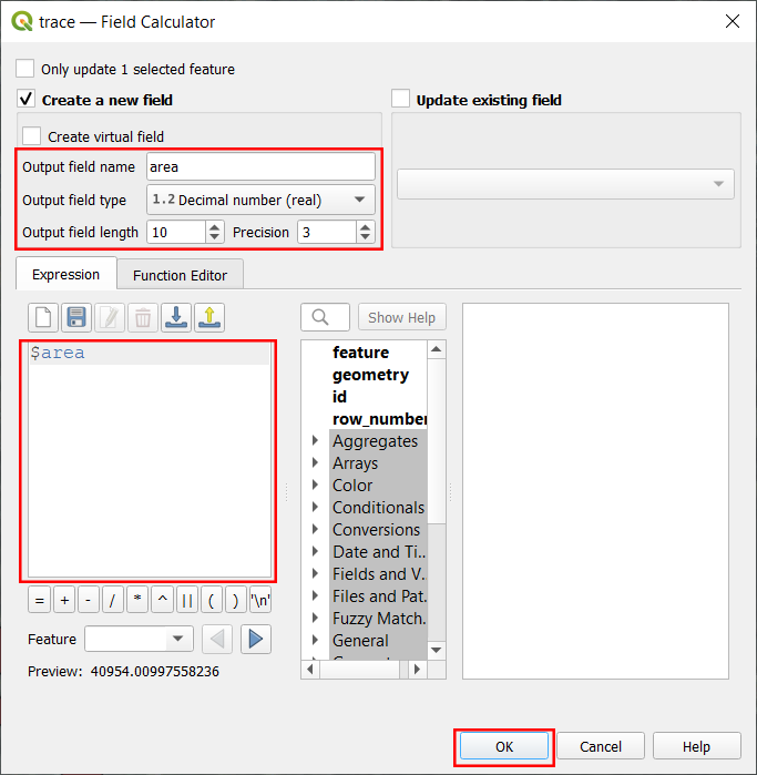
3. Then in the Expression tab input $area or in the middle column open the Geometry tab and click $area.
4. Click OK. If you are not already in Edit mode, you will be prompted to enable it. Do so.
5. Once the calculation is complete, right-click on the layer and select “Open Attribute Table”. View Screenshot

   

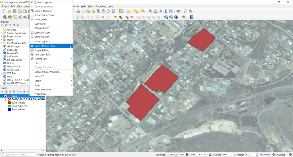
6. You should see an additional field containing the area of each shape. View Screenshot

   

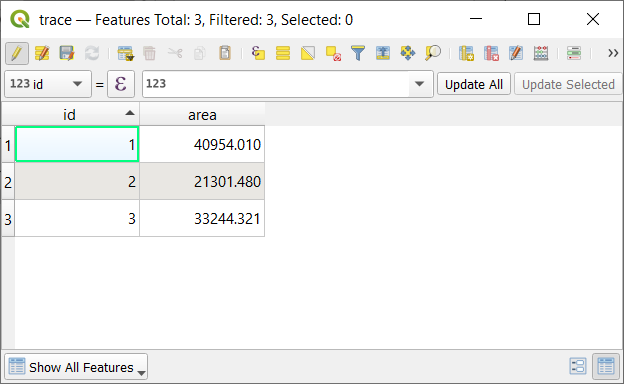
7. If you make a change to the shapes and wish to recalculate the areas, reopen the field calculator window” and check “Update existing field”. Then, in the dropdown box select the area field. Input $area under Expression, and click OK.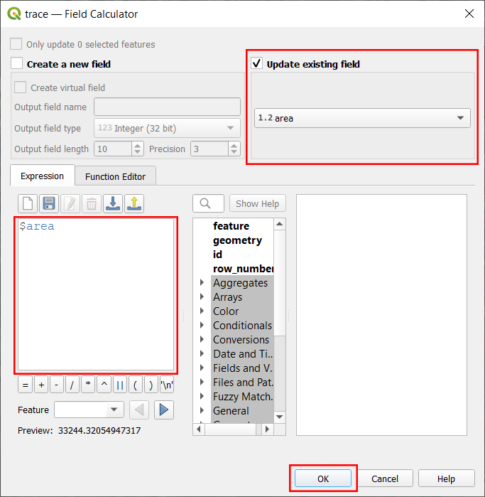 View Screenshot

   

Topographic Lines ↔ DEM

Topographic Lines to DEM

1. Import your contour lines into QGIS. Then, open the Processing Toolbox and search for and double-click on the TIN Interpolation Tool. View Screenshot

   

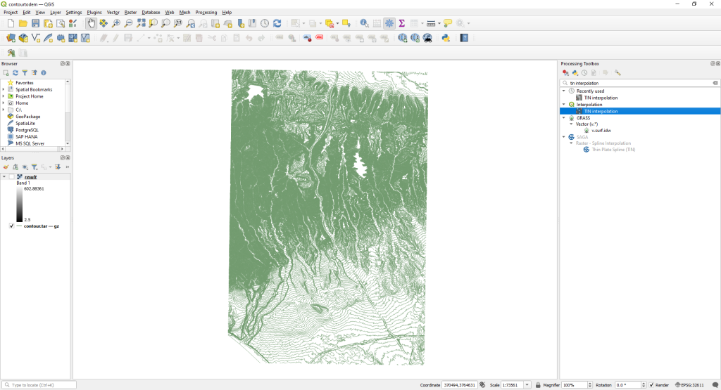
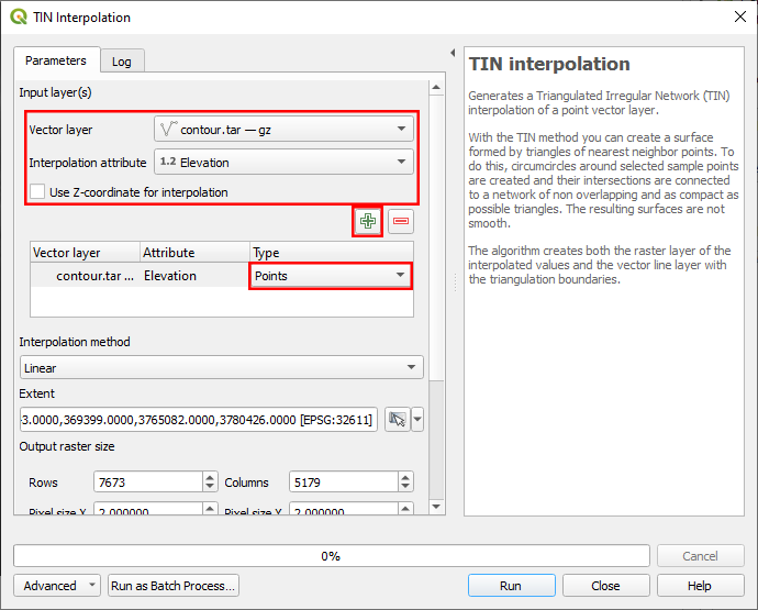
2. In the window, select the contour layer as the “vector layer”, and either enter the field corresponding to elevation as the “interpolation attribute”, or check the box to use the Z-coordinates for that layer. Then, click the green plus and leave Points beneath Type. If you have additional contours or shapes that represent structure or break lines (e.g. cliff or lake boundaries), change the “vector layer” and “interpolation attribute” as required, click the green plus to add it in, and select either “Structure line” or “Break line” under Type. View Screenshot

   

3. Scrolling down, expand the options beneath Extent, and select the option appropriate for where you want to create the DEM. We will use Calculate from Layer to get the DEM to range over the whole layer. View Screenshot

   

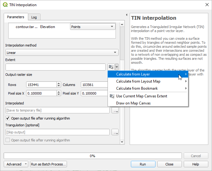
4. Under Output raster size, adjust the pixel size so that the number of displayed rows and columns is not exceedingly large. This will ensure that QGIS will not take too long to produce the output, and that the output DEM file will not be too large. However, note that increasing the size too high will mean the resulting raster will have less precision and follow the contours less. You may want to repeatedly adjust the setting and rerun the algorithm until you are happy with the end result.
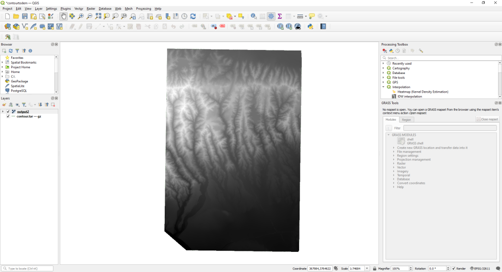
5. Make sure to save the resulting layer by clicking on the three dots underneath Interpolated, then click Run. When the process is finished, a new layer containing the DEM should appear: View Screenshot

   

DEM to Topographic Lines

1. In the menus, click through Raster > Extraction > Contour….
2. In the window, select your DEM layer under “Input layer”, and adjust the value under “Interval between contour lines” as needed. View Screenshot

   

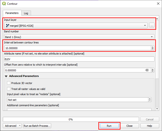
3. Click Run. When the process is done, a new layer will be created containing the contours. [Note: This process may take a lot of time, especially if the DEM covers a large area. You can try increasing the interval between contour lines to shorten the time needed.]
4. To find the elevation of a specific contour line, select the contour layer in the Layers List, and click on the line with the Identify Features tool selected. View Screenshot

   

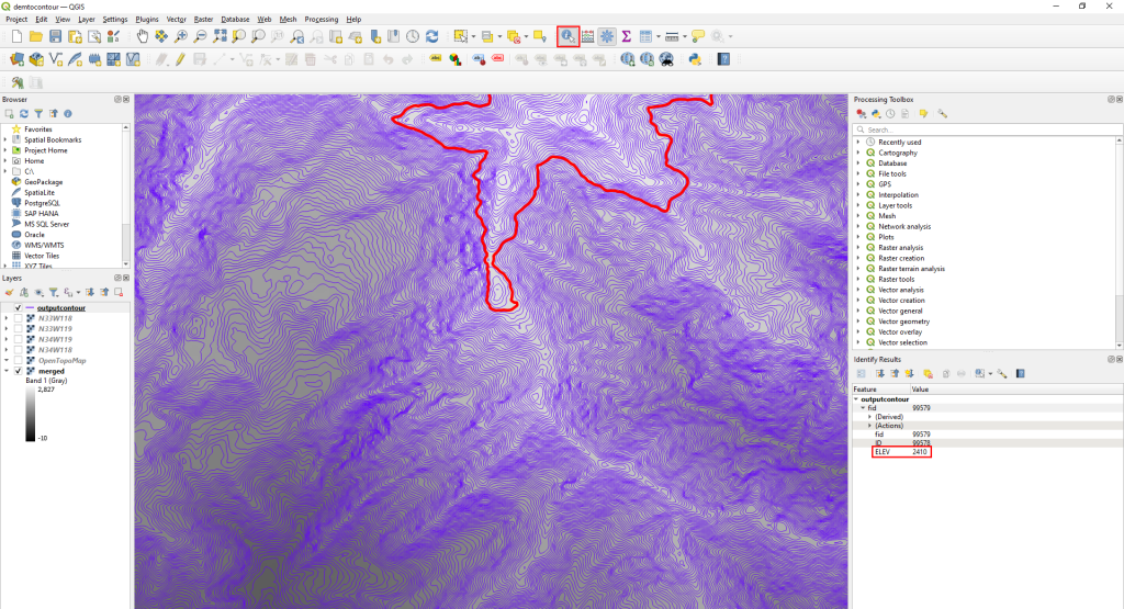
Least Cost Path

1. Create a shapefile layer to add the paths you want to calculate the least cost path over. (If you need a refresher, see Tracing in QGIS). Make sure you add a field for the direction of each path if your network has one-way paths, and a field for speed if you would like to calculate the fastest route. View Screenshot

   

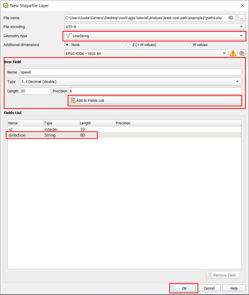
2. Set the new layer to edit mode, and then trace the paths needed. Enter new id values for each. In the direction field, label the path “two-way” if it is two-way, “forward” if it is one-way in the direction you drew the path, or “backward” if it is one-way opposite the direction you drew the path. If you have a speed field, enter the speed of traveling over that path in km/h.
3. When you are done, save your edits and turn off edit mode.
4. Optional: Adding arrows to one-way roads to keep track of path directions
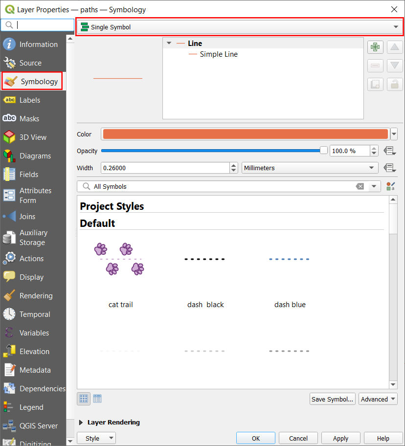
   1. Right-click on the shapes layer and click Properties.
   2. Open the Symbology Tab, click the top dropdown box and select “Rule-based” View Screenshot

      

   3. Click on the green plus “Add rule” button .
   4. In the edit rule window, click the “Expression Editor” icon besides “Filter,” and directly enter the formula “direction” in (‘forward’, ‘backward’)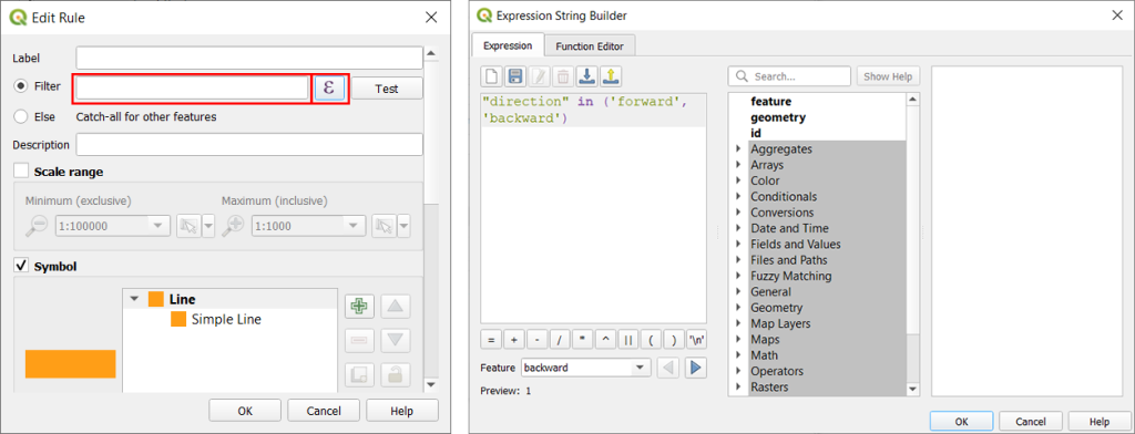View Screenshot

      

   5. This will filter what we do to affect only the one-way roads.
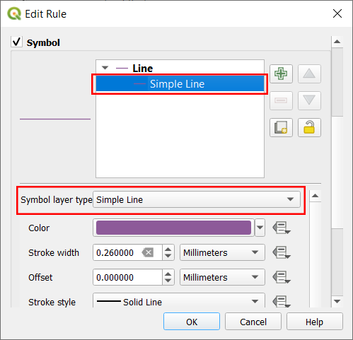
   6. Scroll down to under “Symbol.” Click to select the row “Simple Line,” and then click on the dropdown box beside “Symbol layer type” to choose “Marker Line.” View Screenshot

      

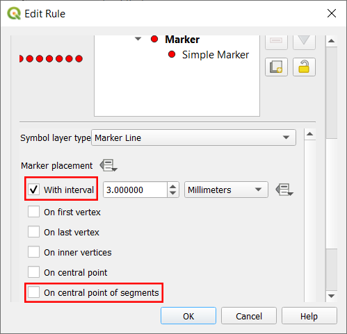
   7. Scroll down further, uncheck “With Interval” and check “On central point of segments” under “Marker Placement” View Screenshot

      

   8. Click and select the bottom-most row labeled “Simple Marker” View Screenshot

      

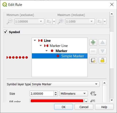
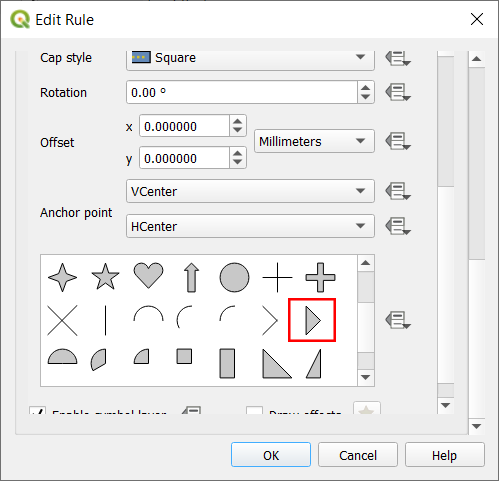
   9. Scroll down to the box of symbols and click on the triangle pointing right. View Screenshot

      

   10. Click on the data-defined override icon in the row for Rotation, and then click Edit.
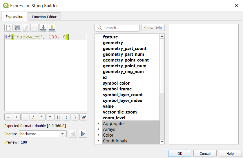
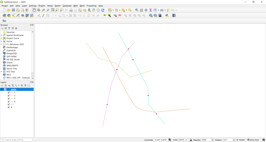
   11. In the Expression Builder, enter if(‘backward’, 180, 0). This will rotate the arrow direction to be in the correct orientation. Then click OK. View Screenshot

       

   12. Finally, click OK to close the “Edit Rule” window, and then click Apply in the Layer Properties Window. You should see arrows along one-way paths traveling in the correct directions. View Screenshot

       

5. Open the Processing Toolbox with the Processing Toolbox icon on the toolbar, or through Processing > Toolbox.
6. In the Processing Toolbox, navigate under “Vector Overlay” to the Split with Lines tool, or search using the search bar. Double left-click to open the dialog. View Screenshot

   

7. In the window that pops up, press Run. A new layer called “Split” should appear that merges all of your paths together. If you have special symbology for your paths, you can turn that layer invisible by checking the box next to it.
8. Then, open the Network Analysis tab in the Processing Toolbox or search to find the “Shortest path (point to point)” tool. Double left-click to open the dialog. View Screenshot

   

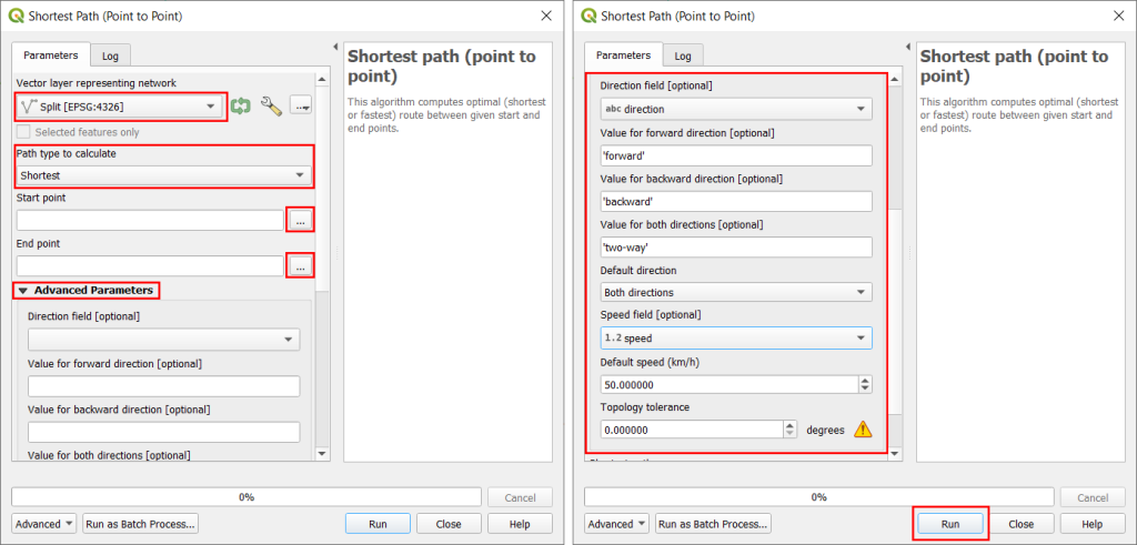
9. Enter the “Split” layer as the “Vector layer representing network”, and select “Shortest” or “Fastest” under “Path type to calculate” based on what you want to compute. Then, click on the three dots besides “Start point” and “End point” to select the points on the network you want to compute an optimal path between.
10. Open the Advanced parameters, and input the direction field and the values used to indicate forward direction, backward direction, and both directions. (See screenshot above). If you are computing the “Fastest” path, you will need to input the speed field also. Click Run.
11. A new layer named “Shortest path” will appear. Open its Attribute table to see the “cost” of the path: distance if you computed the “Shortest” path, or time if your computed the “Fastest” path.

Viewsheds

1. Install the Visibility Analysis Plugin (if you need a refresher on installing plugins, see the instructions here).
2. Import DEM data for the area you want to perform your analysis around. If you don’t already have that data, you can download it from NASA, from the Consortium for Spatial Information, or other sources. If you have topographic contours, you can try converting it to DEM.
3. If you need multiple DEM granules, merge them together through Raster > Miscellaneous > Merge and selecting the layers with the three dots besides “Input layers.” Click Run. Use the outputted layer for the following steps. View Screenshot

   

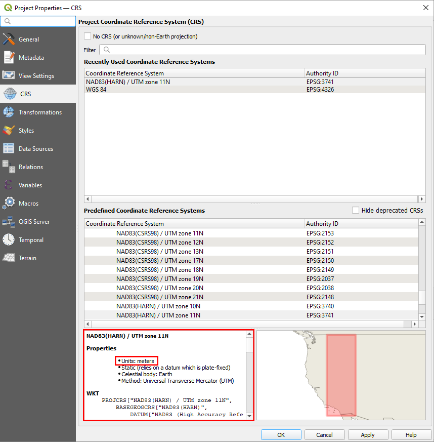
4. Your CRS will also need to have units of meters. If you are unsure if this is the case, click on the globe at the bottom right, and in the window check that your CRS has “meters” as units. View Screenshot

   

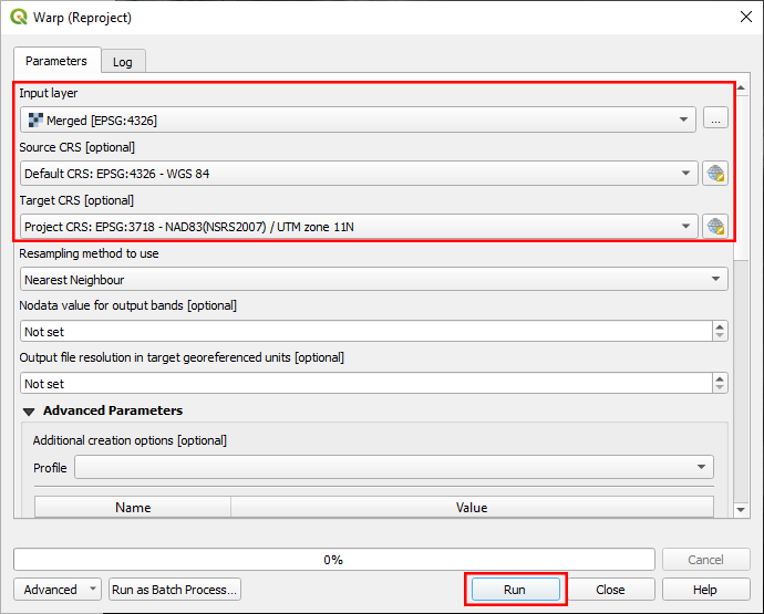
5. If not, you will need to reproject your DEM and data to a CRS that does have meters as units. When you have chosen a CRS, reproject your DEM data by navigating to Raster > Projections > Warp (Reproject). In the window, select the DEM layer, put in the source CRS and target CRS, and then click Run. Use the outputted “Reprojected” layer for the remaining steps. View Screenshot

   

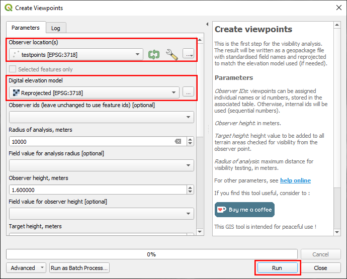
6. Open the Processing Toolbox and select the Create Viewpoints tool from the Visibility Analysis plugin. Under “Observer Location(s)” select a shapefile corresponding to points you want to calculate the viewshed from. Put in the reprojected DEM layer under “Digital Elevation Model.” Fill out the remaining parameters as needed. Click Run. View Screenshot

   

7. In the Processing Toolbox, now select the Viewshed tool. Leave “Analysis type” and “Combining multiple outputs” as is, select the output of the Create Viewpoints tool for “Observer location(s)” and select the reprojected DEM layer for the “Digital elevation model.” Check the box to take into account Earth curvature if you are working over large distances. Then hit Run. You should have an output raster file that gives pixels an integer value corresponding to the number of viewpoints that can “see” that point.

Cluster Analyses

There are two major algorithms in QGIS used for clustering: DBSCAN clustering and K-means clustering.

DBSCAN (Density-based spatial clustering of applications with noise) clusters based on the density of points. Points which are too far away from others are deemed noise and are not clustered.

K-means tries to create a specified number of equal-sized clusters by computing “mean” points and clustering points which are closest to a specific “mean.”

DBSCAN

Make sure that the CRS of your points has units of meters. If not, you may have to reproject (see here).

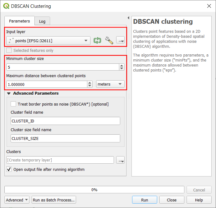
1. In the Processing Toolbox , open the DBSCAN Clustering process.
2. Select your point layer as the Input layer. Then, you will need to adjust the minimum cluster size and maximum distance between clustered points, which determine how “dense” points need to be to form a cluster. View Screenshot

   

3. A new layer should appear. Open the Symbology tab of the Properties window and set the coloring to be done based on CLUSTER_ID (see here for more detailed instructions) to see the clusters (and noise). You may want to adjust the parameters and rerun the DBSCAN algorithm to get better results.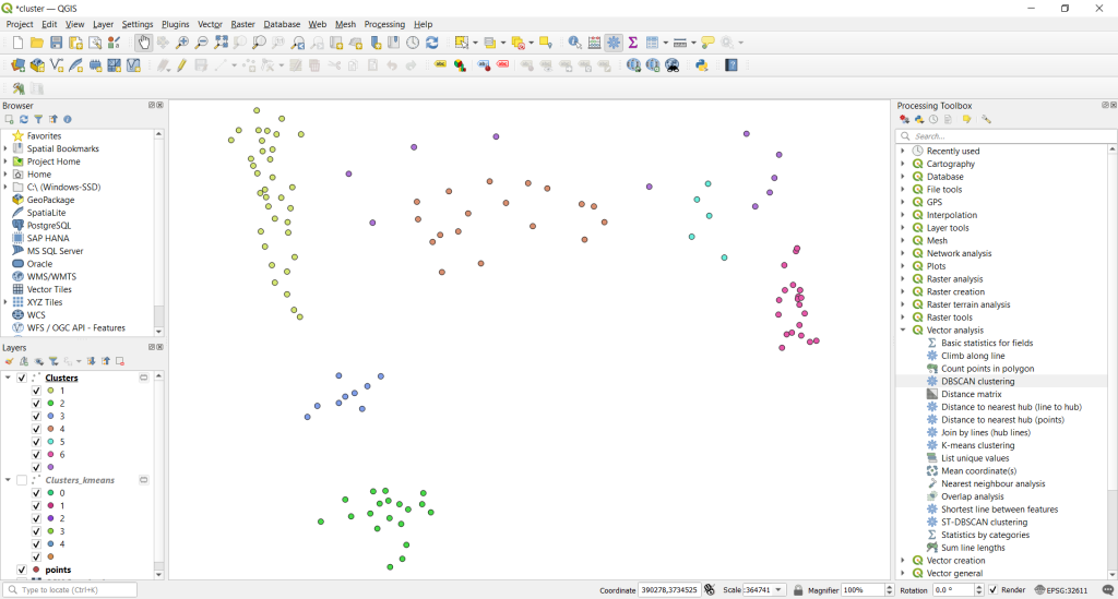 View Screenshot

   

If you are having trouble finding a good distance value for the algorithm, you may want to use the Measure Line tool in the Attributes Toolbar to get a sense for the distances between your points. The parameter “maximum distance between points” determines a radius around every point that the algorithm checks for other points in to determine density, i.e. you may want to measure distances between individual points.

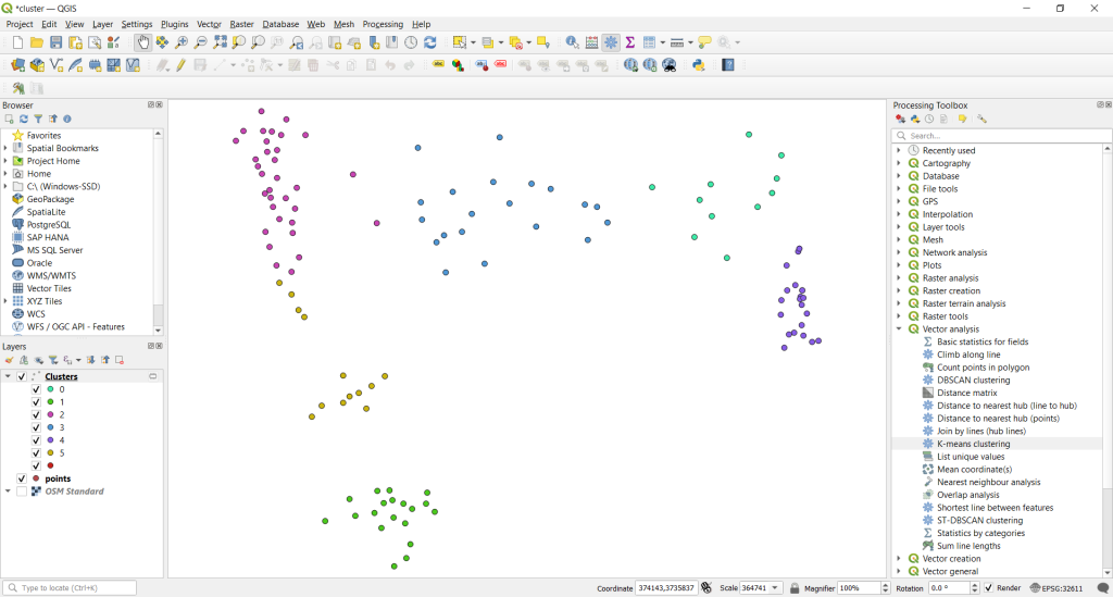
K-means

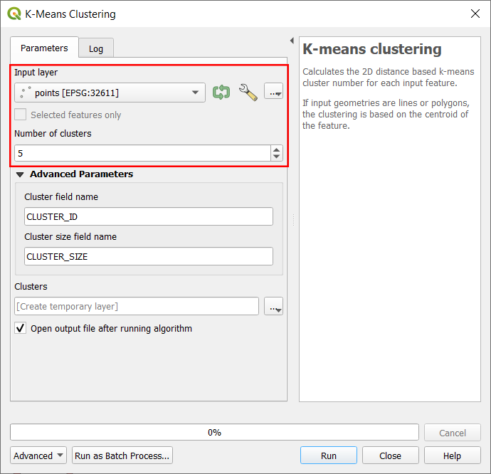
1. In the Processing Toolbox , open the K-means clustering process.
2. In the K-means algorithm window, select your point layer as the input layer, and then input the number of clusters the algorithm should produce. You will probably need to guess and rerun the algorithm multiple times until you are satisfied with the results. View Screenshot

   

3. In the new layer, open the Properties tab and in the Symbology tab, set the coloring to be done based on CLUSTER_ID (see here for more detailed instructions).This will show all of the generated clusters: View Screenshot

   

---

Back to previous page.